4. Monte Carlo Model of Radical Polymerization#
4.1. 📖 Introduction#
As explained in Notebook 2, stochastic methods can also be used (and are sometimes preferable) for simulating polymerization systems. To illustrate this approach, we reimplement the radical polymerization model from Notebook 3 using the Kinetic Monte Carlo (KMC) method.
4.2. 🎲 Algorithm Implementation#
The implementation closely follows the general principles outlined in Notebook 2. The main difference is that the reaction system now includes macromolecular species \(R^{\cdot}_i\) and \(P_i\), whose chain length distribution (CLD) we want to track. For that purpose, in addition to storing the total number of each of these species in the molecule count vector \(X\), we compute and store their respective chain lengths in an additional list. That information is then used after the simulation is completed to reconstruct the full CLD.
import matplotlib.pyplot as plt
import numpy as np
from numba import jit
from numpy.typing import NDArray
For better readability, we define symbolic indices for the different species and reaction types used in the simulation. These indices will make the code more intuitive and reduce the likelihood of errors when referencing specific components.
iX_M = 0   # Monomer
iX_I = 1   # Initiator
iX_R = 2   # Radical
iX_P = 3   # Polymer

ir_p  = 0  # Propagation
ir_d  = 1  # Initiator decomposition
ir_tc = 2  # Termination by combination
ir_td = 3  # Termination by disproportion
The stochastic algorithm is implemented in simulate_polymerization, following the six steps outlined in Notebook 2. Due to the inherently low radical-to-monomer concentration ratio \([R^{\cdot}]/[M]\) in radical polymerizations, the simulation must consider a very large number (\(>10^8\)) of initial monomer molecules to accurately represent the radical population. This large number of molecules results in a proportionally high number of time steps. Therefore, an efficient implementation is essential, and the function is JIT-compiled with Numba to improve performance.
@jit(fastmath=True)
def simulate_polymerization(
    C0: NDArray[np.float64],
    kd: float,
    f: float,
    kp: float,
    ktc: float,
    ktd: float,
    tend: float,
    XM0: int,
    number_snapshots: int = 100
) -> tuple:
    """Simulate batch radical polymerization using Kinetic Monte Carlo.

    Parameters
    ----------
    C0 : NDArray[np.float64]
        Initial concentration vector (mol/L).
    kd : float
        Initiator decomposition rate coefficient (1/s).
    f : float
        Initiation efficiency.
    kp : float
        Propagation rate coefficient (L/(mol·s)).
    ktc : float
        Termination by combination rate coefficient (L/(mol·s)).
    ktd : float
        Termination by disproportionation rate coefficient (L/(mol·s)).
    tend : float
        End simulation time (s).
    XM0 : int
        Initial number of monomer molecules.
    number_snapshots : int
        Number of state snapshots to be stored.

    Returns
    -------
    tuple
        t, V, X, C, Ri, Pi
    """

    # Constants
    NA = 6.022e23

    # Initialize system state
    t = 0.0
    X: NDArray[np.int64] = np.rint(XM0 / C0[iX_M] * C0).astype(np.int64)
    V: float = X[iX_M] / (C0[iX_M]*NA)
    Ri = [0]
    Ri.pop()  # trick to help numba infer the type of Ri
    Pi = [0]
    Pi.pop()

    # Store initial state
    t_trajectory = [t]
    X_trajectory = [X.copy()]
    V_trajectory = [V]
    Ri_trajectory = [Ri.copy()]
    Pi_trajectory = [Pi.copy()]

    # Termination coefficients
    kt = ktc + ktd
    alpha = ktd/kt

    # Start loop
    a = np.zeros(4)
    while True:

        # Rescale rate coefficients
        kd_mc = kd
        kp_mc = kp/(NA*V)
        kt_mc = 2*(kt/2)/(NA*V)

        # Evaluate reaction propensities
        a[ir_d] = kd_mc*X[iX_I]
        a[ir_p] = kp_mc*X[iX_R]*X[iX_M]
        at = kt_mc*X[iX_R]*(X[iX_R] - 1)
        a[ir_tc] = at*(1 - alpha)
        a[ir_td] = at*alpha

        # Select reaction
        a_cumsum = np.cumsum(a)
        a_sum = a_cumsum[-1]
        rand_rxn = np.random.rand()*a_sum
        idx_selected_rxn = np.searchsorted(a_cumsum, rand_rxn)

        # Update number of molecules, chain lengths and volume change
        if idx_selected_rxn == ir_d:
            X[iX_I] -= 1
            ΔV = 0.0
            if np.random.rand() > f:
                X[iX_M] -= 2
                X[iX_R] += 2
                Ri.append(1)
                Ri.append(1)
                ΔV = 0.0
        elif idx_selected_rxn == ir_p:
            X[iX_M] -= 1
            idx_Ri = np.random.randint(len(Ri))
            Ri[idx_Ri] += 1
            ΔV = 0.0
        elif idx_selected_rxn == ir_tc:
            X[iX_R] -= 2
            X[iX_P] += 1
            idx_Ri = np.random.randint(len(Ri))
            Pi_ = Ri[idx_Ri]
            Ri.pop(idx_Ri)
            idx_Ri = np.random.randint(len(Ri))
            Pi_ += Ri[idx_Ri]
            Ri.pop(idx_Ri)
            Pi.append(Pi_)
            ΔV = 0.0
        elif idx_selected_rxn == ir_td:
            X[iX_R] -= 2
            X[iX_P] += 2
            for _ in range(2):
                idx_Ri = np.random.randint(len(Ri))
                Pi.append(Ri[idx_Ri])
                Ri.pop(idx_Ri)
            ΔV = 0.0
        else:
            raise ValueError("Invalid reaction index.")

        # Update volume
        V += ΔV

        # Elapsed time
        rand_tau = np.random.rand()
        if a_sum > 0.0:
            tau = (1/a_sum)*np.log(1/rand_tau)
        else:
            tau = tend - t
        t += tau

        #  Store state snapshot
        if (t/tend*number_snapshots - 1 > len(t_trajectory)):
            t_trajectory.append(t)
            X_trajectory.append(X.copy())
            V_trajectory.append(V)
            Ri_trajectory.append(Ri.copy())
            Pi_trajectory.append(Pi.copy())

        # Stop if end time reached or no more monomer molecules
        if t >= tend or X[iX_M] == 0 or X[iX_I] == 0:
            break

    # Convert to numpy arrays
    t_ = np.asarray(t_trajectory)
    V_ = np.asarray(V_trajectory)
    X_ = np.empty((len(X_trajectory), X_trajectory[0].size), dtype=np.int64)
    for i in range(len(X_trajectory)):
        X_[i, :] = X_trajectory[i]
    Ri_ = [np.array(x) for x in Ri_trajectory]
    Pi_ = [np.array(x) for x in Pi_trajectory]

    # Compute molar species concentrations
    C_ = X_/(V_[:, np.newaxis]*NA)

    return t_, V_, X_, C_, Ri_, Pi_
4.3. 📊 Results and Visualization#
4.3.1. Runing the Simulation#
For consistency, we use the same parameters as in Notebook 3. However, feel free to experiment with them!
f = 0.5
kd = 4e-4  # 1/s
kp = 4e3   # L/(mol·s)
ktc = 1e8  # L/(mol·s)
ktd = 1e8  # L/(mol·s)

C0 = np.zeros(4)
C0[iX_M] = 1e0  # mol/L
C0[iX_I] = 1e-2 # mol/L

tend = 3.6e3  # s
The initial number of monomer molecules is set to \(10^8\) to keep the computation time within reasonable bounds. For more accurate results, consider increasing this number to around \(10^9\).
t, V, X, C, Ri, Pi = \
    simulate_polymerization(C0, kd, f, kp, ktc, ktd, tend, XM0=10**8)
On my computer, a simulation with \(10^8\) molecules takes around 9 seconds. Since computation time scales linearly with the system size, a simulation with \(10^9\) monomer molecules takes about 1.5 minutes, which is still quite reasonable.
4.3.2. Species Concentrations#
Let’s start by visualizing the time evolution of the molar concentrations of all species. For polymeric species, this corresponds to their zeroth moment.
fig1, ax = plt.subplots(4, 1, sharex=True, figsize=(7, 4*2))
fig1.suptitle("Species Concentrations")
fig1.tight_layout()
fig1.align_ylabels()

for idx, species in zip([iX_I, iX_M, iX_R, iX_P], ['I', 'M', 'R*', 'P']):
    ax[idx].plot(t, C[:, idx])
    ax[idx].set_ylabel(f"[{species}] (mol/L)")
    ax[idx].grid(True)

ax[-1].set_xlabel("Time (s)");
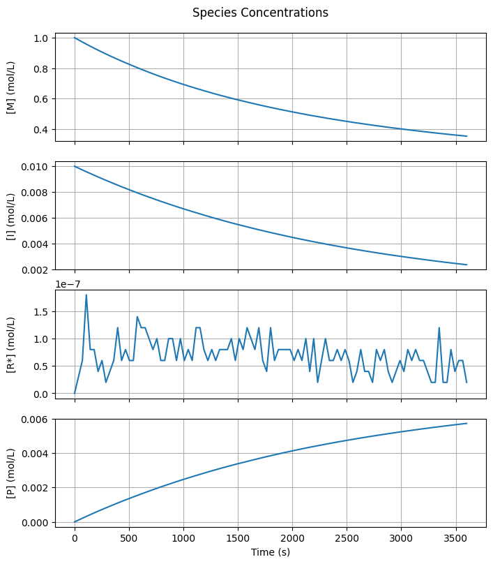
Note that the \([R^{\cdot}]\) curve is particularly noisy, while the other curves appear smooth. This noise is a direct consequence of the very low steady-state radical concentration (~\(10^{-7}\) mol/L), which corresponds to just \(10^1\) radicals in a simulation with \(10^8\) monomer molecules.
4.3.3. Average Chain Lengths#
The leading moments of the radical and dead polymer distributions can be calculated from the lengths of the individual chains. From these, the number- and mass-average degrees of polymerization and the polydispersity index can be computed.
def moment(Q: list[np.ndarray], m: int) -> np.ndarray:
    "m-th moment of `Q`"
    if m == 0:
        result = [q.size for q in Q]
    elif m == 1:
        result = [q.sum() for q in Q]
    else:
        result = [np.sum(q**m) for q in Q]
    return np.array(result)
moment_R = [moment(Ri, m) for m in range(3)]
moment_P = [moment(Pi, m) for m in range(3)]
fig2, ax = plt.subplots(2, 1, sharex=True, figsize=(7, 2*2))
fig2.suptitle("Average Chain Lengths & Dispersity")
fig2.tight_layout()
fig2.align_ylabels()

for moment, name in zip([moment_R, moment_P], ["R*", "P"]):
    DPi = moment[1]/(moment[0] + 1e-10)
    DPw = moment[2]/(moment[1] + 1e-10)
    PDI = DPw/(DPi + 1e-10)
    ax[0].plot(t, DPi, label=name)
    ax[1].plot(t, PDI, label=name)
    ax[0].set_ylabel(r"$DP_{\mathrm{n}}$")
    ax[1].set_ylabel(r"$PDI$")
    ax[0].grid(True)
    ax[1].grid(True)

ax[0].legend(loc='upper right')
ax[-1].set_xlabel("Time (s)");
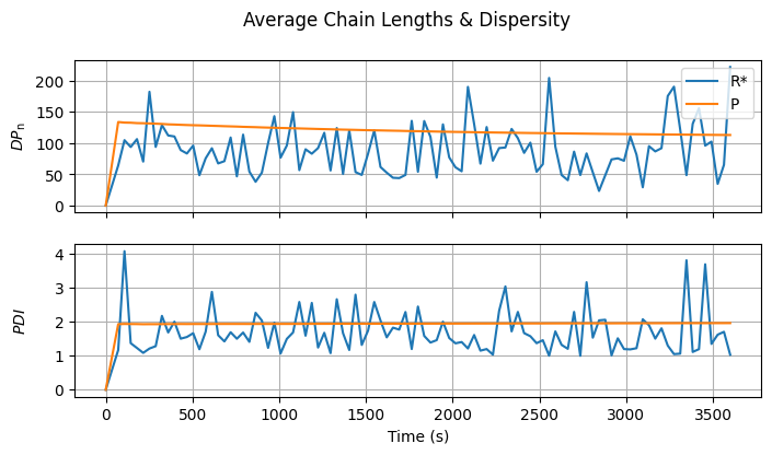
The values are plausible for both distributions, though significantly noisy for \(R^{\cdot}\) due to the small radical sample. You may want to set ktc or ktd to zero and observe how this affects the average chain length and polydispersity index of the dead polymer.
4.3.4. Chain Length Distribution#
Last but not least, we can try to reconstruct the full chain length distributions of \(R^{\cdot}\) and \(P\).
fig3, ax = plt.subplots(2, 1, sharex=True, figsize=(7, 2*2))
fig3.suptitle("Chain Length Distributions")
fig3.tight_layout()
fig3.align_ylabels()

for i, (Y, Yname) in enumerate(zip([Ri, Pi], [r"$R^{\cdot}(i)$", r"$P(i)$"])):
    for ii in [1, int(0.25*len(t)), int(0.5*len(t)), int(0.75*len(t)), -1]:
        y, x = np.histogram(Y[ii], bins=40, density=False)
        x = (x[:-1] + x[1:])/2
        y = y/y.max()
        label = f"t={t[ii]:.1e} s"
        ax[i].plot(x, y, label=label)

    ax[i].set_ylabel(Yname)
    ax[i].grid(True)

ax[0].legend(loc='best')
ax[-1].set_xlabel("Chain length");
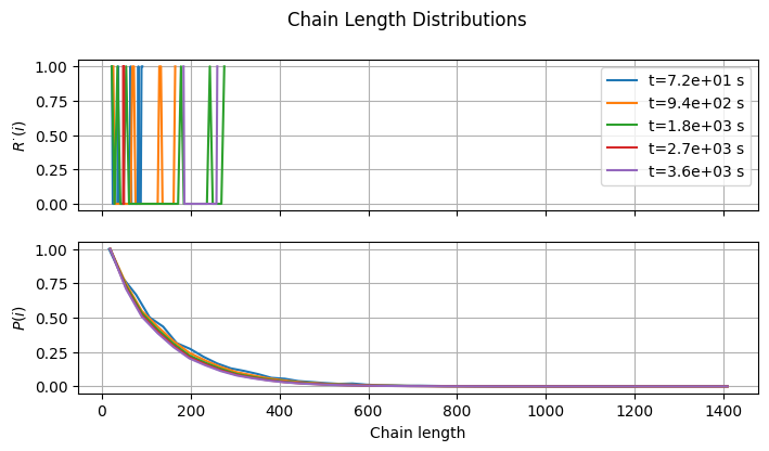
The dead polymer CLD exhibits the expected Flory-like shape. In contrast, the radical CLD is unrecognizable. To obtain a meaningful curve, a significantly larger radical count would be required. If you have time and RAM to spare, you can give it a try…
4.4. 🔎 Questions#
Based on this example, how would you evaluate the performance of the KMC method for radical polymerization and, more generally, for reaction systems with low-concentration transient species?
The accuracy of the stochastic simulation can be improved not only by increasing
XM0, but also by running multiple simulations with lowerXM0and combining their results. Implement this approach.