3. Discrete Population Balance Model of Radical Polymerization#
3.1. 📖 Introduction#
Radical polymerization (RP) is a type of chain-growth polymerization in which the active center is a radical. The reaction mechanism involves at least three key steps: initiation, propagation, and termination. In this case, the reaction scheme can be written as follows:
where \(I\) is the initiator, \(M\) is the monomer, \(R_i^{\cdot}\) is a radical chain of length \(i\), \(P_i\) is a (dead) polymer chain of length \(i\), \(k_{\mathrm{d}}\) is the initiator decomposition rate coefficient, \(k_{\mathrm{p}}\) is the propagation rate coefficient, and \(k_{\mathrm{tc}}\) and \(k_{\mathrm{td}}\) are the rate coefficients for termination by combination and disproportionation, respectively.
For a closed system with constant volume and constant rate coefficients, the corresponding transient species balances are:
By defining an appropriate upper limit for the chain length \(N\), we obtain a closed system of \(2N+2\) ordinary differential equations (ODEs). However, numerically solving this ODE system is challenging. Under typical polymerization conditions, very long chains are formed, requiring rather large \(N\) values (possibly \(10^4\)–\(10^5\) or higher). Moreover, the presence of short-lived radical species makes the ODE system stiff, requiring implicit solvers.
Special numerical methods are therefore needed to solve the population balances efficiently and stably. You can read about it here. In this tutorial, we integrate the discrete population balances directly. This brute-force approach is quite inefficient (be prepared to wait 10–60 s, depending on CPU performance), but it serves a pedagogical purpose by providing transparency in its workings.
3.2. 🧮 Model Implementation#
3.2.1. Architecture#
Before diving into the code, the diagram below provides a high-level overview of the model architecture: solve_model calls SciPy’s solve_ivp, which repeatedly evaluates model_xdot, and model_xdot in turn delegates the differential balances to the individual reaction submodels.
        graph TD
    solve_model[solve_model]
    solve_ivp[solve_ivp]
    model_xdot[model_xdot]
    initiation[initiation]
    propagation[propagation]
    termination[termination]

    solve_model --> solve_ivp
    solve_ivp --> model_xdot
    model_xdot --> initiation
    model_xdot --> propagation
    model_xdot --> termination
3.2.2. Code Implementation#
import matplotlib.pyplot as plt
import numpy as np
from numba import jit, prange
from scipy.integrate import solve_ivp
We begin by implementing separate functions to compute the differential mole balances for the three reaction steps: initiation, propagation, and termination. All functions are JIT-compiled with Numba to improve performance.
Numba
When used properly, Numba can generate highly optimized machine code, achieving performance close to that of statically typed languages. However, debugging Numba-decorated functions can be challenging. Therefore, it is best to activate Numba only after ensuring that the underlying Python function works as intended.
@jit(fastmath=True)
def initiation(
    I: float,
    M: float,
    kd: float,
    f: float
) -> tuple[float, float, float]:
    """Initiation balances.

    I -> 2 I*      , kd
    I* + M -> R(1) , fast

    d[I]/dt = -kd*[I]
    d[M]/dt = -2*f*kd*[I]
    d[R(1)]/dt = 2*f*kd*[I]

    Parameters
    ----------
    I : float
        Initiator concentration.
    M : float
        Monomer concentration.
    kd : float
        Initiator decomposition rate coefficient.
    f : float
        Initiation efficiency.

    Returns
    -------
    tuple[float, float, float]
        Molar balances for I, M and R(1).
    """
    Idot = -kd*I
    ri = 2*f*kd*I*(M/(M + 1e-10))
    Mdot = -ri
    R1dot = ri
    return Idot, Mdot, R1dot
@jit(fastmath=True, parallel=True)
def propagation(
    R: np.ndarray,
    M: float,
    kp: float
) -> tuple[float, np.ndarray]:
    """Propagation balances.

    R(i) + M -> R(i+1) , kp

    d[R(i)]/dt = kp*[M]*([R(i-1)] - [R(i)])
    d[M]/dt = -kp*[M]*sum([R(i)])

    Parameters
    ----------
    R : np.ndarray
        Radical concentrations.
    M : float
        Monomer concentration.
    kp : float
        Propagation rate coefficient.

    Returns
    -------
    tuple[float, np.ndarray]
        Molar balances for M and Rn.
    """
    Mdot = -kp*M*R.sum()
    Rdot = np.zeros_like(R)
    for i in prange(1, R.size):
        Rdot[i] = kp*M*(R[i-1] - R[i])
    return Mdot, Rdot
@jit(fastmath=True, parallel=True)
def termination(
    R: np.ndarray,
    ktc: float,
    ktd: float
) -> tuple[float, np.ndarray]:
    """Termination balances.

    R(i) + R(j) -> P(i+j)      , ktc
    R(i) + R(j) -> P(i) + P(j) , ktd

    d[R(i)]/dt = -2*(ktc + ktd)*[R(i)]*[R]
    d[P(i)]/dt = ktc * sum j=1:i-1 [R(i-j)]*[R(j)] + 2*ktd*[R(i)]*[R]

    Parameters
    ----------
    R : np.ndarray
        Radical concentrations.
    ktc : float
        Termination by combination rate coefficient.
    ktd : float
        Termination by disproportionation rate coefficient.

    Returns
    -------
    tuple[float, np.ndarray]
        Molar balances for Rn and Pn.
    """
    # d[R(i)]/dt
    Rdot = -2*(ktc + ktd)*R*R.sum()
    # d[P(i)]/dt
    Pdot = np.zeros_like(R)
    if ktc > 0.0:
        for n in prange(2, R.size):
            accum = 0.0
            for i in range(1, n):
                accum += R[i]*R[n-i]
            Pdot[n] = accum
        Pdot *= ktc
    Pdot += 2*ktd*R*R.sum()
    return Rdot, Pdot
Next, we combine all the reaction steps into a function that evaluates the total rate of change of the state vector \(\boldsymbol{x}\), which contains the concentrations of all species.
@jit(fastmath=True, parallel=True)
def model_xdot(
    t: float,
    x: np.ndarray,
    kd: float,
    kp: float,
    ktc: float,
    ktd: float,
    f: float,
    N: int
) -> np.ndarray:
    """Calculate derivative of the state vector, dx/dt.

    x = [I, M, R_0..R_N, P_0..P_N]

    Parameters
    ----------
    t : float
        Time.
    x : np.ndarray
        State vector.
    kd : float
        Initiator decomposition rate coefficient.
    kp : float
        Propagation rate coefficient.
    ktc : float
        Termination by combination rate coefficient.
    ktd : float
        Termination by disproportionation rate coefficient.
    f : float
        Initiation efficiency.
    N : int
        Maximum chain length.

    Returns
    -------
    np.ndarray
        Time derivative of the state vector.
    """
    # Unpack the state vector
    I = x[0]
    M = x[1]
    R = x[2:N+3]
    # P = y[N+3:]

    # Compute the kinetic steps
    Idot, Mdot, R1dot = initiation(I, M, kd, f)
    Mdot_, Rdot = propagation(R, M, kp)
    Mdot += Mdot_
    Rdot_, Pdot = termination(R, ktc, ktd)
    Rdot += Rdot_
    Rdot[1] += R1dot

    # Assemble the derivative vector
    xdot = np.empty_like(x)
    xdot[0] = Idot
    xdot[1] = Mdot
    xdot[2:N+3] = Rdot
    xdot[N+3:] = Pdot

    return xdot
Finally, we perform the numerical integration using a suitable ODE solver. This system is very stiff, therefore we need to chose an implicit solver like LSODA.
def solve_model(
    I0: float,
    M0: float,
    kd: float,
    f: float,
    kp: float,
    ktc: float,
    ktd: float,
    N: int,
    tend: float
) -> tuple[np.ndarray, ...]:
    """Solve the dynamic model.

    Parameters
    ----------
    I0 : float
        Initial initiator concentration (mol/L).
    M0 : float
        Initial monomer concentration (mol/L).
    kd : float
        Initiator decomposition rate coefficient (1/s).
    f : float
        Initiation efficiency.
    kp : float
        Propagation rate coefficient (L/(mol·s)).
    ktc : float
        Termination by combination rate coefficient (L/(mol·s)).
    ktd : float
        Termination by disproportionation rate coefficient (L/(mol·s)).
    N : int
        Maximum chain length.
    tend : float
        End time (s).

    Returns
    -------
    tuple[np.ndarray, ...]
        Time, chain lengths, I, M, R(i), P(i).
    """

    # Chain lengths (include length 0, to make indexing easier)
    s = np.arange(0, N+1)

    # Initial conditions
    R0 = np.zeros_like(s)
    P0 = np.zeros_like(s)
    x0 = np.concatenate(([I0], [M0], R0, P0))

    # Solve ODE set
    teval = np.linspace(0.0, tend, num=100+1)
    atol = np.concatenate(
        ([1e-6], [1e-6], 1e-11*np.ones_like(R0), 1e-7*np.ones_like(P0)))

    solution = solve_ivp(model_xdot,
                         t_span=(0.0, tend),
                         y0=x0,
                         t_eval=teval,
                         args=(kd, kp, ktc, ktd, f, N),
                         method='LSODA',  # implicit solver is a MUST
                         rtol=1e-3,
                         atol=atol)

    # Unpack the solution
    t = solution.t
    x = solution.y
    I = x[0, :]
    M = x[1, :]
    R = x[2:N+3, :]
    P = x[N+3:, :]

    return t, s, I, M, R, P
3.3. 📊 Results and Visualization#
3.3.1. Runing the Simulation#
Let’s start with some educated guesses, while being carefull not to make very long chains.
# Parameters
f = 0.5
kd = 4e-4  # 1/s
kp = 4e3   # L/(mol·s)
ktc = 1e8  # L/(mol·s)
ktd = 1e8  # L/(mol·s)

# Initial concentrations
M0 = 1.0   # mol/L
I0 = 1e-2  # mol/L

# Simulation time
tend = 3600  # s

# Maximum chain length
N = 1000
The initial kinetic chain length informs us about the average degree of polymerization of the macroradicals. N must be well above this value, otherwise chains escape the numerical domain.
kinetic_chain_length = kp/(2*np.sqrt(f*kd*(ktc+ktd))) * M0/np.sqrt(I0)

print(f"The kinetic chain length is {kinetic_chain_length:.0f}.")
if (N < 5*kinetic_chain_length):
    answer = "insufficient"
else:
    answer = "sufficient"
print(f"N={N} appears {answer}.")
The kinetic chain length is 100.
N=1000 appears sufficient.
Here we go! This might take a while, depending on how large \(N\) is.
t, s, I, M, R, P = solve_model(I0, M0, kd, f, kp, ktc, ktd, N, tend)
By the way, can you pinpoint which part of the code is the rate-limiting step?
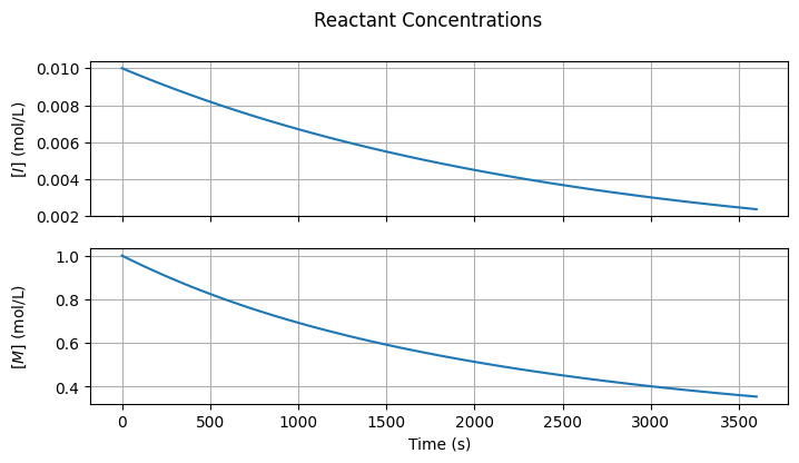
3.3.2. Reactant Concentrations#
Below are visualizations showing how the initiator and monomer concentrations evolve over time.
fig1, ax = plt.subplots(2, 1, sharex=True, figsize=(7, 2*2))
fig1.suptitle("Reactant Concentrations")
fig1.tight_layout()
fig1.align_ylabels()

# [I] on the first subplot
ax[0].plot(t, I)
ax[0].set_ylabel(r"$[I]$" + " (mol/L)")
ax[0].grid(True)

# [M] on the second subplot
ax[1].plot(t, M)
ax[1].set_ylabel(r"$[M]$" + " (mol/L)")
ax[1].grid(True)

ax[-1].set_xlabel("Time (s)");
3.3.3. Moments#
Below are visualizations that show how the characteristic moments and related averages of the radical and polymer distributions evolve over time.
def moment(Q: np.ndarray, m: int) -> np.ndarray:
    "m-th moment of `Q`"
    s = np.arange(0, Q.shape[0])
    return np.dot(s**m, Q)
fig2, ax = plt.subplots(4, 1, sharex=True, figsize=(7, 4*2))
fig2.suptitle("Moments of R* and P")
fig2.tight_layout()
fig2.align_ylabels()

eps = np.finfo(float).eps

# 0-th moment of R*
r0 = moment(R, 0)
ax[0].plot(t, r0)
ax[0].set_ylabel(r"$[R^{\cdot}]$" + " (mol/L)")
ax[0].grid(True)

# Number-average degree of polymerization of R*
r1 = moment(R, 1)
DPn_R = r1 / (r0 + eps)
ax[1].plot(t, DPn_R)
ax[1].set_ylabel(r"$DP_{\mathrm{n}}(R^{\cdot})$")
ax[1].grid(True)

# 1st moment of P
p1 = moment(P, 1)
ax[2].plot(t, p1)
ax[2].set_ylabel(r"$\lambda_1(P)$")
ax[2].grid(True)

# Number-average degree of polymerization of P
p0 = moment(P, 0)
DPn = p1 / (p0 + eps)
ax[3].plot(t, DPn)
ax[3].set_ylabel(r"$DP_{\mathrm{n}}(P)$")
ax[3].grid(True)

ax[-1].set_xlabel("Time (s)")

mass_balance_error = np.max(np.abs((r1 + p1 + M)/M0 - 1.0))
print(f"Mass balance error: {mass_balance_error:.1e}")
Mass balance error: 3.1e-04
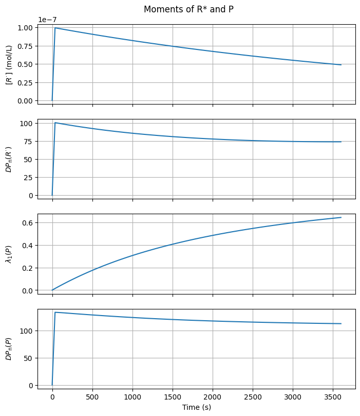
The mass balance error is of the same order as the relative tolerance specified in the ODE solver, suggesting that the solution is consistent.
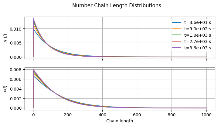
3.3.4. Chain Length Distribution#
And finally, the number chain length distributions of the radicals and dead polymer.
fig3, ax = plt.subplots(2, 1, sharex=True, figsize=(7, 2*2))
fig3.suptitle("Number Chain Length Distributions")
fig3.tight_layout()
fig3.align_ylabels()

# Normalize Rn and Pn by peak and plot them
for i, (Y, Yname) in enumerate(zip([R, P], [r"$R^{\cdot}(i)$", r"$P(i)$"])):
    for ii in [1, int(0.25*len(t)), int(0.5*len(t)), int(0.75*len(t)), -1]:
        y = Y[:, ii].copy()
        y /= (y.sum() + eps)
        ax[i].plot(s, y, label=f"t={t[ii]:.1e} s")
    ax[i].set_ylabel(Yname)
    ax[i].grid(True)

ax[0].legend(loc="best")
ax[-1].set_xlabel("Chain length");
3.4. 🔎 Questions#
What is the relationship between the average degree of polymerization of \(R^{\cdot}\) and \(P\)?
What is the physical meaning of the 1st moment of \(P\)?
What system property did we use to check the mass balance error?
What kind of distribution does \(R^{\cdot}\) follow? And what about \(P\)?
Calculate \([R^{\cdot}]\) using the quasi-steady state approximation, and compare it to the value obtained by solving the transient radical balances.